You can find the paper in Optics Express.
Dynamic Full Field OCT (D-FFOCT) is very promising for 4D microscopy with diffraction limited resolution and also for eye imaging. In this paper we present two methods, (i) a Singular Value Decomposition (SVD) based filtering method that automatically removes artifact arising from sample axial motion during the acquisition, and (ii) a new operator based on non-stationnarities to compute the dynamic image in order to improve the Signal to Noise Ratio (SNR). While the first method is a great step toward in vivo D-FFOCT imaging the second method allow deeper imaging in scattering media. Finally we report on the first in vivo dynamic acquisition on a living mouse liver.
SVD filtering for motion artifact removal
Theoretical considerations
One drawback of DFFOCT lies in its main advantage, it has a nanometer sensitivity. This means that the slightest mechanical vibration will cause a tremendous signal variation compared to the typical probed fluctuations. Indeed, the static sample reflexion coefficient is typically two order of magnitude higher than the metabolic fluctuations. This means that mechanical vibration can bury the signal of interests under high artifacts. This was not really an issue in the lab because the setup is mounted on a sturdy optical bench that filter out most of the vibrations. Problems arise when clinicians try to use such system in very noisy environment (mechanical vibrations, air conditionning, etc.) and for in vivo imaging. Therefore, these artifacts need to be filtered out in order to retrieve the metabolic image.
So basically when we acquire a DFFOCT stack we end up with the summation of our signal of interest - which is very small- and the signals arising from motion artifacts - which is typicaly very strong -. Our goal is then to separate those two contributions in order to retrieve only the motility term.
Proposed algorithm
In order to un-mix the artifactual signals we used the SVD which is the generalization of the eigendecomposition of a positive semidefinite normal matrix, and can be thought of as decomposing a matrix into a weighted, ordered sum of separable matrices which will become handy when reconstructing the denoised signals:
\[M_u = U\Sigma V^\star = \sum _ { i } \sigma _ { i } \mathbf { U } _ { i } \otimes \mathbf { V } _ { i }\]where $\otimes$ is the outer product operator, $U$ contains the spatial eigenvectors, $V$ contains the temporal eigenvectors and $\Sigma$ contains the eigenvalues associated with spatial and temporal eigenvectors. Performing the SVD on an unfolded $M_u(1440\times 1440,512)$ dynamic stack takes around 30 seconds on a workstation computer (Intel i7-7820X CPU, 128 Gbyte of DDR4 2666 MHz RAM) and requires 45 GByte of available RAM using LAPACK routine for SVD computation without computing full matrices. Investigating such decomposition for artifact-free data sets we found that spatial eigenvectors related to motion artifacts have particular and easily identifiable associated temporal eigenvectors. Indeed, when looking at the first temporal eigenvectors, we observed sinusoid-like patterns with increasing frequency. In presence of motion artifacts, temporal eigenvectors appeared with random, high-frequency components that are easy to detect with simple features. Here, the zero crossing rate (the number of times a function crosses $y=0$) is used to detect temporal eigenvectors involved in motion artifacts. In presence of motion artifacts some of the firsts temporal eigenvectors present a high zero crossing rate. In order to detect these outliers we computed the absolute value of the derivative of the zero crossing rate (D-ZRC $= |ZRC_{i+1}-ZRC_{i}|$) and applied a threshold: if the D-ZRC is higher than three times the D-ZRC standard deviation then the corresponding eigenvalue $\sigma_i$ is set to zero in $\hat{\Sigma}$ and the SVD-denoised stack $\hat{M}_u$ is reconstructed as:
\[\hat{M}_u = \sum _ { i } \hat{\sigma _ { i }} \mathbf { U } _ { i } \otimes \mathbf { V } _ { i }\]The SVD-denoised stack $\hat{M}_u$ can then be folded back to its original 3D shape $\hat{M}$ and the dynamic computation can be performed. Interestingly, the use of an automatic selection of eigenvectors allows a more reproducible analysis. For example, the SVD can be performed on spatial sub-regions without visible artifacts, something very hard to obtain with manual selection of eigenvectors. This can also improve the filtering procedure in the case of sample spatial deformation or if the computation requires too much RAM.
Results
Applying the proposed method on clinical data taken on cancerous lung biopsies we show that it reduces effectively artifacts arising from highly reflective structures motion:
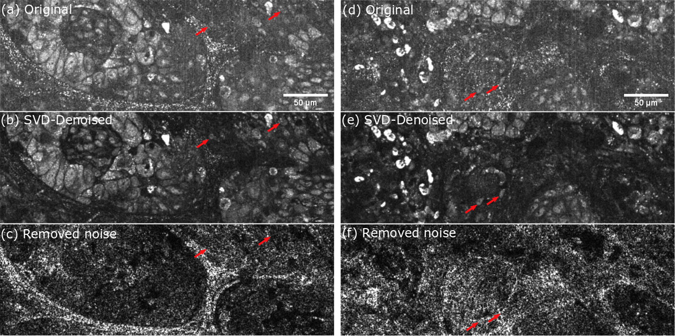 Lung biopsy for cancer detection taken on the LLTech clinical setup. Artifacts arise mainly from mechanical vibration and air conditioning. (a)(d) Original D-FFOCT images computed on the raw stack. (b)(e) Denoised images computed with SVD filtering. (c)(f) Sum of the spatial eigenvectors absolute value removed by the SVD filtering. Red arrows are highlighting cells that were partially masked by motion artifacts.
Cumulative sum for deeper imaging
In addition to motion artifacts, a drawback of D-FFOCT compared to standard static FFOCT is the reduced penetration depth. While FFOCT can acquire images as deep as $1~mm$, D-FFOCT is limited to about $100~\mu m$ due to the weak signal level produced by the sample fluctuations we wish to measure. In order to enhance the dynamic signal strength and so improve penetration depth, we propose computation of the dynamic image from the cumulative sum of the signal, rather than the raw signal. Indeed, the model for the dynamic image formation is small scatterers moving in the coherence volume during the acquisition leading to phase and amplitude fluctuations in the conjugated camera pixel. While a pure Brownian motion is stationary, hyper-diffusive displacements are not and we therefore propose to use the cumulative sum to enhance these non-stationarities. Intuitively, summing a centered noise will give a noisy trajectory that stays close to zero whereas if there is a small bias it will be summed for every sample and the cumulative sum will therefore have a slope equal to this bias.
Let us consider an array of random values drawn from a zero centered Gaussian distribution. If the number of samples is large the mean of the array will be close to zero and equivalently the sum of all the samples will also be close to zero. Taking the cumulative sum of such an array gives a so called Brownian bridge (the curve starts and ends close to zero and makes a “bridge” between these two points). Theoretically, Brownian bridges are expected to be maximal close to the edges as the probability distribution of the maximum is the third arcsin law which has a typical U-shape. More importantly, the Brownian bridge maximum follows a Rayleigh distribution. If we consider a Brownian bridge $W_s ~ \forall ~ s \in [0,1]$:
\[W_M=sup\{W_s:s\in [0,1]\}\] \[\mathbb { P } [ W_M \leq u ] = 1 - e^{ - 2 u ^ { 2 }}\]where $W_M$ is the supremum of the bridge and $\mathbb { P } [ W_M \leq u ]$ is the probability of the supremum being less than $u$. According to the Rayleigh distribution, the Brownian bridge maximum must therefore scale as $\sqrt{t}$ with $t$ scaling as the number of frames. Now, if there is a bias in the distribution, which is the case if a scatterer is moving with constant velocity in the coherence volume, the cumulative sum will scale as $\frac{t}{2}$ due to the slope introduced by the bias. It will also be either always positive or negative and the maximum will be reached around the center of the bridge. The cumulative sum will therefore exhibit a completely different behavior for centered noise than for actual motility signals, leading to a better signal to noise ratio on dynamic images. Note that for Brownian bridges it is often observed that the function changes sign regularly (the probability of sign changes is also well established, which is not the case when there are non-stationarities.
Results
The dynamic image is computed by taking the average of the maxima of the absolute values of the running cumulative sum:
\[I'_{dyn}(\boldsymbol{r}) =\frac{1}{N} \sum_i max\left(|CumSum\left(I(\boldsymbol{r},t_{[i, i+\tau]})-\bar{I}(\boldsymbol{r},t_{[i, i+\tau]})\right)|\right)\]where $CumSum$ is the cumulative sum operator, $N$ is the total number of sub-windows, $\tau$ is the sub-windows length so that $t_{[i,i+\tau]}$ is the time corresponding to one sub-window and $\bar{I}(\boldsymbol{r},t_{[i, i+\tau]})$ is the signal mean on the sub-window. We tested the proposed method with $\tau=50$ on the photoreceptor layer of an explanted macaque retina at $85~\mu m$ depth that presents a horizontal gradient of SNR.
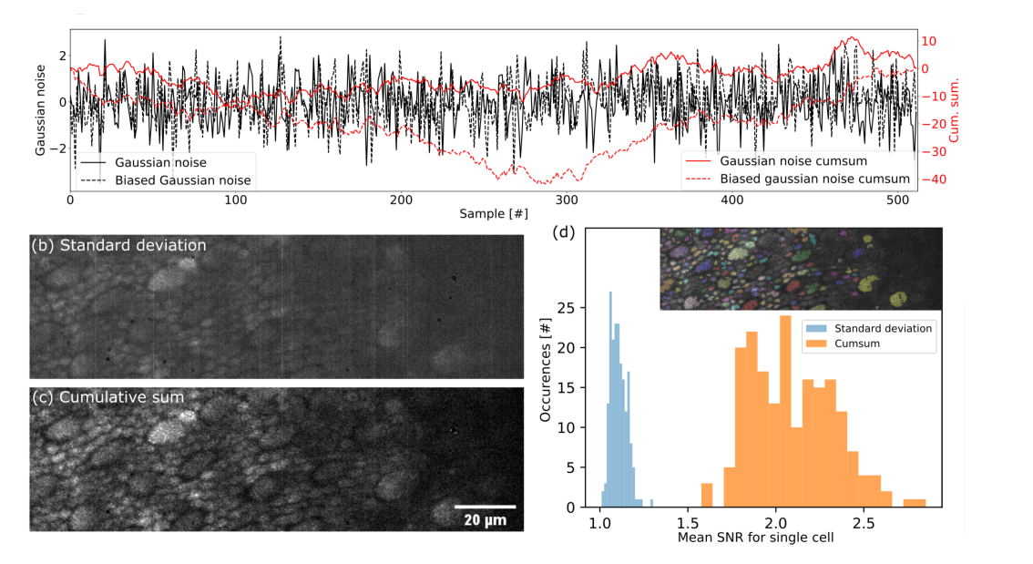 (a) Simulation of Gaussian noise with and without bias and their cumulative sum. The maximum reached by the cumulative sum is 3 times higher with the bias. (b) Dynamic image of a macaque photoreceptor layer using standard deviation. (c) Dynamic image of a macaque photoreceptor layer using the proposed method based on cumulative sum. (d) Histogram of SNR for 192 single cells segmented in (b) and (c). Segmentation results are shown in the top right corner. The gain in SNR for this data set is 1.96 on average for each cell.